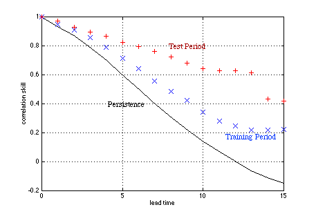
Figure 1. The correlation skill of the neural network model.
We are continually trying to improve the forecasts by our neural network models. Recently, we have advanced on the instability problem, namely that the forecasts made by neural network models using different training initialization and different data vary considerably, though all with similar skills. One of the causes is that the neural network model has too many weights, i.e., too many connections among neurons.
We thus applied different methods to prune the networks. One method we implemented is called Optimal Brain Damage (OBD). In OBD, the importance of each weight is judged by the cost function (measuring the model error) increase when the weight is removed. Then the weight that causes the least cost function increase is removed and the network is retrained. This procedure continues until only 3 weights are left. As the network is being pruned, its performance is evaluated on both the training data and the test data, which are set aside from the training. Usually, as the network is pruned, the error on the training data (the cost function in the training) increases, and the error on the test data decreases to a minimum and then increases again.
To our surprise, that minimum in error on the test data turned out to occur when the neural network had been pruned to an extremely simple one, consisting of only one hidden neuron, and 3 inputs. The connections to other inputs and other neurons of the neural network were all pruned away. The resulting network has only 4 weights in the following form
x1(t + leadtime) = w4 tanh( w1 x1 + w2 x2+ w3 x3),where w1, w2, w3 and w4 are the 4 weights, whose values depend on the leadtime, and listed in Table 1, and x1, x2, and x3 are the NINO3.4 index (from http://nic.fb4.noaa.gov/data/cddb/), the 2nd and the 3nd EOF coefficients of the FSU monthly wind stress data (Goldenberg and O'Brien 1981). Before the EOF calculation, the wind data were first smoothed with one pass of a 1-2-1 filter in the zonal and meridional directions and in time, and detrended and de-seasoned by subtracting from a given month the average of the same calendar months of the previous four years. This pre-EOF processing is the same as that used in Lamont's coupled model (Cane et al. 1986) and in Tang (1995).
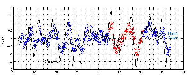
We set the NINO3.4 and wind stress data from 1961 to 1981 and from 1991 to 1996 as training data, and the data from 1982 to 1990 as test data. The reason of this division is that the test period consists of 2 warm events and 2 cold events, so it is easy to see the strength of a trained model in forecasting an event. This active test period has a higher signal/noise ratio than the training period, which may boost the test skills shown in Fig. 1. Figure 2 is the comparison of the observed NINO3.4 and the model output at the 6-month leadtime. The correlation skills are 0.64, 0.81, 0.69 for the training period, test period, and the two period combined, respectively.
We compared this pruned neural network with a linear regression model consisting of the same input and output. For the 3 month leadtime, the two are almost identical. For the 6 month leadtime, the neural network is about 0.03 higher in correlation skill. While for the 9 month leadtime, the skills are almost the same again. The small weights shown in Table 1 reveal that the neural network does not go much into the nonlinear regime.
We have also developed a pruned neural network model for the COADS SLP data, which has higher skills than the present model of FSU wind for longer leadtimes (Tangang et al, 1997). However, due to the lack of a consistent, long, and timely updated SLP data set, we are unable to issue real time forecast with that model at the present time.

Figure 1. The correlation skill of the neural network model.

Figure 2. Comparison between the observed NINO3.4 (solid line) and the model output at a 6-month leadtime (circles). The difference between the two in the training period (1961 to 1981, and 1991 to 1996) was minimized during the training. The model forecasts during the training period is indicated by blue circles, and during the test period by red circles. The tick mark on the time axis indicates January 1 of the year.
leadtime        w1        w2        w3        w4
       3     -0.2725   -0.0911    0.0908   -2.9908
       6     -0.3162   -0.2558    0.2424   -1.6744
       9     -0.1715   -0.4628    0.3741   -1.0595
Cane, M.A., S.E. Zebiak and S. Dolan, 1986: Experimental forecasts of El Nino. Nature, 321, 827-832.
Goldenberg, S.B., and J.J. O'Brien, 1981: Time and space variability of tropical Pacific wind stress. Mon. Wea. Rev., 109, 1190-1207.
Tang, B., 1995: Periods of linear development of the ENSO cycle and POP forecast experiments. J. Climate, 8, 682-691.
Tangang, F.T., W.W. Hsieh and B. Tang, 1997: Forecasting the equatorial Pacific see surface temperatures by neural network models. Climate Dynamics, to appear.