Download our recent paper entitled " 'Clearning' Neural Networks with Continuity Constraint for Prediction of Noisy Time Series" ([in postscript format, 84K])
Normally, when a neural network is trained, only the network weights are adjusted to minimize a cost function which measures only the difference between the network output and the data. In our data assimilating neural network, not only the weights, but also the network input are adjusted. The cost function to be minimized consists of three terms. The first term is the cost function of a traditional neural network, measuring the difference between the network output and the data (the output constraint). The second term measures the difference between the network input and the data (the input constraint). It was proposed by Weigend et al (1996), and was termed "clearning", after the words "learning" and "cleaning", meaning that the neural network learns from the data and cleans the data at the same time. The third term measures the difference between the network output and the network input for the next step (continuity constraint). It acts as a weak constraint of continuity, forcing the end of one step to be close to the beginning of the next step. When training is finished, forecast starts from the network output for the starting month obtained in the training, instead of from the raw data, similar to initialization by adjoint data assimilation.
The data used for training are the NINO3 SST index and the first 4 EOF coefficients of the FSU monthly wind stress data (Goldenberg and O'Brien 1981). The seasonal cycle, calculated from the 1961 to 1990 data, has been remove from the NINO3 data. Before the EOF calculation, the wind data were first smoothed with one pass of a 1-2-1 filter in zonal and meridional directions and in time, and detrended and de-seasoned by subtracting from a given month the average of the same calendar months of the previous four years. This pre-EOF processing is the same as that used in Lamont's coupled model (Cane et al 1986) and in Tang (1995).
The inputs of the neural network for a given month consist of the NINO3 index and the first 4 wind EOF coefficients of the month and the same 5 numbers for the month that is 3 months earlier, amounting to 10 inputs to the network. These inputs feed into a hidden layer with 4 sigmoidal neurons, which in turn feed into 5 linear output neurons, giving the NINO3 and the first 4 wind EOF coefficients for the month that is 3 months later. Thus, the time step of the neural network is 3 months. By repeatedly feeding the model output as input to the neural network, we can obtain forecasts for longer lead times. The skill of this multiple-step forward feeding is a good check of the predicting power of the neural network.
The neural network has 69 weights to be adjusted, and there are only 420 training pairs in the period from 1961 to 1995. (The number of training pairs is smaller for the retroactive real time forecasts described later.) To prevent overfitting, we implemented a termination scheme. For every 5 training iterations, the training is paused and the neural network is fed forward repeatedly to make hindcasts. The average correlation skills of the 3rd step and the 4th step (9 months and 12 months forward, respectively) is calculated. This long-term skill usually increases with training to a maximum (at about 80 to 100 iterations) but then starts to decrease. The training is terminated at this point of maximum long-term skill, even though the one-step error measured by the cost function is still decreasing.
To estimate the forecast skill, retroactive real time forecasts for January 1986 to September 1995 were carried out, entailing a total of 118 neural network trainings, one for each month.

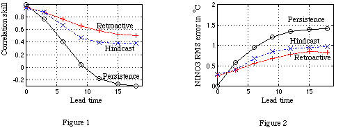
Fig.1 and Fig. 2 show the correlation skill and the RMS error for the retroactive forecast (+) from 1986 to 1995, the hindcast (x) and the persistence (o) for the whole period (1961-1995). The outputs obtained in the training are used to start the feed forward, so that at the initial time the correlation is not one and the RMS error is not zero. The forecast skills are higher than the hindcast skills; other models also tend to give higher skills in the 80's and the 90's. Due to the 1-2-1 filter in time, the initial condition contains information of the next month. Thus, in Figs. 1 and 2, a 3-month lead skill should be interpreted as a 2-month lead skill, etc.
References
Cane, M.A., S.E. Zebiak and S. Dolan, 1986: Experimental forecasts of
El Nino. Nature, 321, 827-832.
Goldenberg, S.B., and J.J. O'Brien, 1981: Time and space variability of tropical Pacific wind stress. Mon. Wea. Rev., 109, 1190-1207.
Tang, B., W. Hsieh and F. Tangang, 1996: "Clearning" neural networks with continuity constraint for prediction of noisy time series. Proceedings of International Conference on Neural Information Processing 1996, Hong Kong, Volume 2, p722-725.
Tang, B., 1995: Periods of linear development of the ENSO cycle and POP forecast experiments. J. Climate, 8, 682-691.
Tang, B., G. Flato and G. Holloway, 1994: A study of Arctic sea ice and sea level pressure using POP and neural network methods. Atmos.-Ocean, 32, 507-529.
Tangang, F. T., W. W. Hsieh and B. Tang, 1995: Forecasting the equatorial Pacific see surface temperatures by neural network models.Climate Dynamics, submitted.
Weigend, A.S, H.G. Zimmermann, and R. Neuneier, 1996: Clearning. Submitted.