After an extensive sensitivity study (Tang et al 1998), we started issuing our NINO3.4 sea surface temperature forecasts with an upgraded (version 2.3) neural network model in May, 1998.
The data in this forecast came from two data sets: the COADS sea level pressure (SLP) data of the tropical Pacific Ocean for latitudes from 20S to 20N (Smith et al. 1996, from ftp://nic.fb4.noaa.gov/pub/ocean/clim1/oimonth), and the NOAA sea surface temperature (SST) data of the tropical Pacific Ocean in latitudes from 30S to 30N (Woodruff et al 1987, from http://www.cdc.noaa.gov/coads/). Both data sets contain monthly 2X2-degree data with time coverage from January 1950 to May 1998.
The gridded SLP and SST data went through several steps of processing. The SLP data were first averaged to a lower resolution of 10 deg. longitude by 4 deg. latitude. Climatological monthly means, calculated from 1950 to 1997, were removed from both data sets. The SLP and SST data were then smoothed by a 3-month running mean. Empirical orthogonal function (EOF) analysis was performed on each of the two data sets for data reduction. The first 7 EOF time series for SLP and the first 10 EOF time series for SST were retained. These retained SLP and SST EOF time series were normalized so they all had the same variance.
For a given month, we stacked the SLP EOF values of 3, 6 and 9 months before this month together with the SLP and SST EOF values of this month. Altogether, this yielded 38 time series. An extended second-step EOF (EEOF) calculation was carried out to reduce the 38 EOF time series to 12 retained EEOF time series.
This 12 EEOF were used as the predictors (inputs) of the neural network model. The output of the neural network model was the NINO3.4 index calculated from the NOAA gridded SST data set mentioned above.
The neural network used here is a simple feedforward neural network, consisting of an input layer for the 12 inputs, a hidden layer of 7 nonlinear units, and an output layer of 1 linear unit. An ensemble of 20 neural networks were trained, each with a different weight initialization. The final model output was the average of the outputs from the 20 members of the ensemble. The reader is referred to Tangang el al (1998) and Hsieh and Tang (1998) for details.
The advantage of the ensemble model is to reduce variance, or instability of the neural network. The error surface of neural network training is full of local minima; trainings with different initial weights are usually trapped in different local minima. These local minima reflect partly the fitting to the regularities of the data and partly the fitting to the noise in the data. Ensemble averaging tends to cancel the noise part as it varies among the ensemble members, and tends to retain the fitting to the regularities of the data.
We have designed a cross-validation scheme to estimate the forecast skill of the NN models. For each lead time from 3 months to 18 months and for each given year from 1950 to 1997, data from a window of 7 years, starting from January of the given year, were withheld. Training pairs were composed from the remaining data. After the model was trained, forecasts were made from the first 5 years of the 7-year window. Then the 7-year window was moved forward by 5 years and the procedure was repeated.
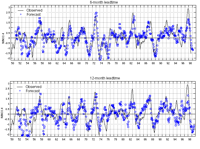
All the forecasts for a given lead time were collected to form a continued forecast NINO3.4 time series. The two panels of Fig. 1 compare the forecast NINO3.4 at leadtimes 6 months and 12 months with the observed NINO3.4. The Correlation coefficients between the forecast and observed NINO3.4 were calculated as skills for each decade from 1950s to 1990s, and for the whole period as well. The results are listed in Table 1.

Table 1. The test correlation skills for different test periods
test period  3-month  6-month  9-month  12-month  15-month
1950-1959      0.72     0.53     0.40     0.36      0.08
1960-1969      0.78     0.63     0.57     0.55      0.43
1970-1979      0.91     0.77     0.72     0.66      0.51
1980-1989      0.85     0.73     0.66     0.71      0.77
1988-1997      0.85     0.69     0.51     0.56      0.55
1950-1997      0.83     0.67     0.56     0.54      0.42
Hsieh, W.W. and B. Tang, 1998: Applying neural network models to prediction and data analysis in meteorology and oceanography. Bull. Am. Meteorol. Soc. Accepted.
Smith, T.M., R.W. Reynolds, R.E. Livezey, and D.C. Stokes, 1996: Reconstruction of historical sea surface temperatures using empirical orthogonal functions. J. Climate, 9, 1403--1420.
Tang, T., W.W. Hsieh, A.H. Monahan and F.T. Tangang, 1998: Seasonal predictions of sea surface temperatures in the tropical Pacific - Comparing neural networks and canonical correlation analysis. J. Climate, submitted.
Tangang, F.T., B.Tang, A.H. Monahan, and W.W. Hsieh, 1998: Forecasting ENSO events: a neural network - extended EOF approach. J. Climate, 11, 29--41.
Woodruff, S.D., R.J. Slutz, R.L. Jenne, and P.M. Steurer, 1987: A comprehensive ocean-atmosphere data set. Bull. Am. Meteorol. Soc., 6, 1239-1250.