A neural network (NN) model has been used by our group to predict the SST anomalies in the Nino3.4 region in the equatorial Pacific (Tang et al. 2000). By version 3.1, the NN model has been extended to forecast the SST anomalies over the whole tropical Pacific. The major difference between this new version 3.2 and version 3.1 is that the subsurface temperature anomalies in the tropical Pacific ocean are now included as predictors.
The data used in this forecast came from three datasets: (a) the monthly sea level pressure (SLP) on 2.5° × 2.5° grids from the NCEP/NCAR reanalysis (Kalnay et al. 1996; downloadable from ftp.cdc.noaa.gov/Datasets/ncep.reanalysis.derived/surface); (b) the monthly extended reconstructed sea surface temperature on 2° × 2° grids (ERSST version 2; Smith and Reynolds 2004; downloadable from ftp.ncdc.noaa.gov/pub/data/ersst-v2); and (c) the monthly 3-dimensional temperatures (called T3 thereafter) in the tropical Pacific ocean from the NCEP Pacific Ocean Analysis (with 1.5° × 1° grids in horizontal and 19 vertical levels in upper 400 meters; Behringer et al. 1998; downloadable from http://ingrid.ldeo.columbia.edu/SOURCES/.NOAA/.NCEP/.EMC/.CMB/.Pacific). The T3 data are available only after January 1980. Anomalies for the SLP, SST and T3 were calculated by subtracting the monthly climatology based on the 1980-2003 period. After applying a 3-month running mean to the gridded data, singular spectrum analysis (SSA) (also known as extended empirical orthogonal function (EEOF) analysis) was performed separately on the three anomaly datasets over the tropical Pacific (SLP: 120°E-70°W, 20°S-20°N; SST: 124°E-70°E, 20°S-20°N; and T3: 122.25°E-71.25°W, 20°S-20°N, 0-345m) with 1-month lags and a 9-month lag window. The predictand is one of the 5 leading principal components (PC) of the SST anomalies over the tropical Pacific, i.e. the SST PCs were predicted separately. The predictors are among the leading SSA PCs of the SLP and those of the SST and T3.
A cross-validation scheme was used to evaluate the forecast skills. The data record (Jan. 1980 - Sept. 2004) was divided into 6 equal segments. Data from one segment were withheld as validation data, while data from the other 5 segments were used to train the models. Thus, independent forecast was made for the period of the validation data using the models based on the training data. This procedure was repeated until all 6 segments were predicted, and the correlation and the root mean square error (RMSE) between the predicted SSTA and the corresponding observed SSTA could be calculated over the whole record. The linear regression (LR) models show that, at 3 months forecast lead time, using 9 SST SSA PCs as predictors performs best; at 6 months lead time, 6 SLP SSA PCs plus 3 T3 SSA PCs; at 9 months, 8 SLP SSA PCs plus 3 T3 SSA PCs; at 12 months, 8 SLP SSA PCs plus 3 T3 SSA PCs; and at 15 months, 7 SLP SSA PCs plus 3 T3 SSA PCs give the best skills (averaged over the whole equatorial Pacific 160°E-70°W, 5°S-5°N).
In the NN models, we used the same predictors and the cross-validation scheme as used in the LR models (for the purpose of comparison). Only 85% of the training data (denoted by D85, randomly chosen from the 5 segments of training data) were used to train the NN model and the remaining 15% (D15) were reserved for an overfitting test. For each set of D85, we made 30 optimization runs to find the model (weight and bias) parameters from random initial parameters, and the run with the smallest mean square error (MSE) was selected and used to make an independent forecast for the data D15. Meanwhile, an LR model was also built on the D85. If the NN model MSE on D15 is less than 1.1*MSE on D85, and less than the MSE from the corresponding LR forecast, the solution was accepted. This entire procedure was repeated 12 times to give 12 models. The average of the predictions from these 12 models are used as the final forecast model. Since there are 6 segments for cross-validation and each segment has 12 models, there is a total of 72 models.
The real time forecast is then made by the ensemble average of all 72 models. It was also found that, for the forecast for the SST PC1, PC4 and PC5, the NN models need only 1 hidden neuron (as using more hidden neurons decreases the skills), while for the forecast for the SST PC2 and PC3, the NN models with multiple hidden neurons (we use 2 at the moment) can have better skills.
The cross-validated forecast skills for the regions Nino4, Nino3.4, Nino3 and Nino1+2 (stretching from the western equatorial Pacific to the eastern equatorial Pacific) are given in the table below. Skills from the LR models are also given for comparison with the NN models.
        |           Correlation           |           RMSE (in °C)
--------|---------------------------------|--------------------------------
   Lead |  Nino4  Nino34   Nino3 Nino1+2  |  Nino4  Nino34   Nino3 Nino1+2
--------|---------------------------------|--------------------------------
      3 |  0.883   0.877   0.841   0.767  |  0.295   0.434   0.515   0.739
      6 |  0.772   0.796   0.749   0.653  |  0.405   0.546   0.634   0.891
NN    9 |  0.725   0.704   0.677   0.593  |  0.440   0.647   0.713   0.972
     12 |  0.593   0.605   0.628   0.541  |  0.540   0.735   0.752   1.011
     15 |  0.449   0.513   0.539   0.418  |  0.588   0.791   0.823   1.113
--------|---------------------------------|--------------------------------
      3 |  0.855   0.877   0.838   0.740  |  0.326   0.433   0.520   0.778
      6 |  0.706   0.761   0.699   0.536  |  0.460   0.591   0.690   1.013
LR    9 |  0.619   0.686   0.659   0.524  |  0.513   0.667   0.733   1.039
     12 |  0.528   0.573   0.591   0.485  |  0.556   0.767   0.802   1.078
     15 |  0.454   0.525   0.546   0.380  |  0.587   0.792   0.829   1.162
--------|---------------------------------|--------------------------------
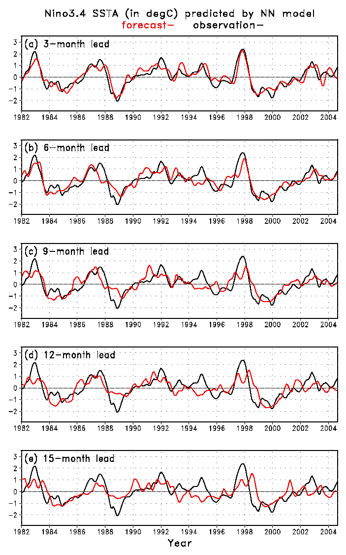
Fig. 1 shows the Nino3.4 SSTA predicted by the NN model against the observations.
Fig. 2 shows the correlation skill (left column) of the NN model at 3-15 month forecast lead times. The difference of the correlation skill between the NN model and the linear regression (LR) model (NN minus LR) is shown in the right column. Areas with positive value (NN better than LR) are shaded.

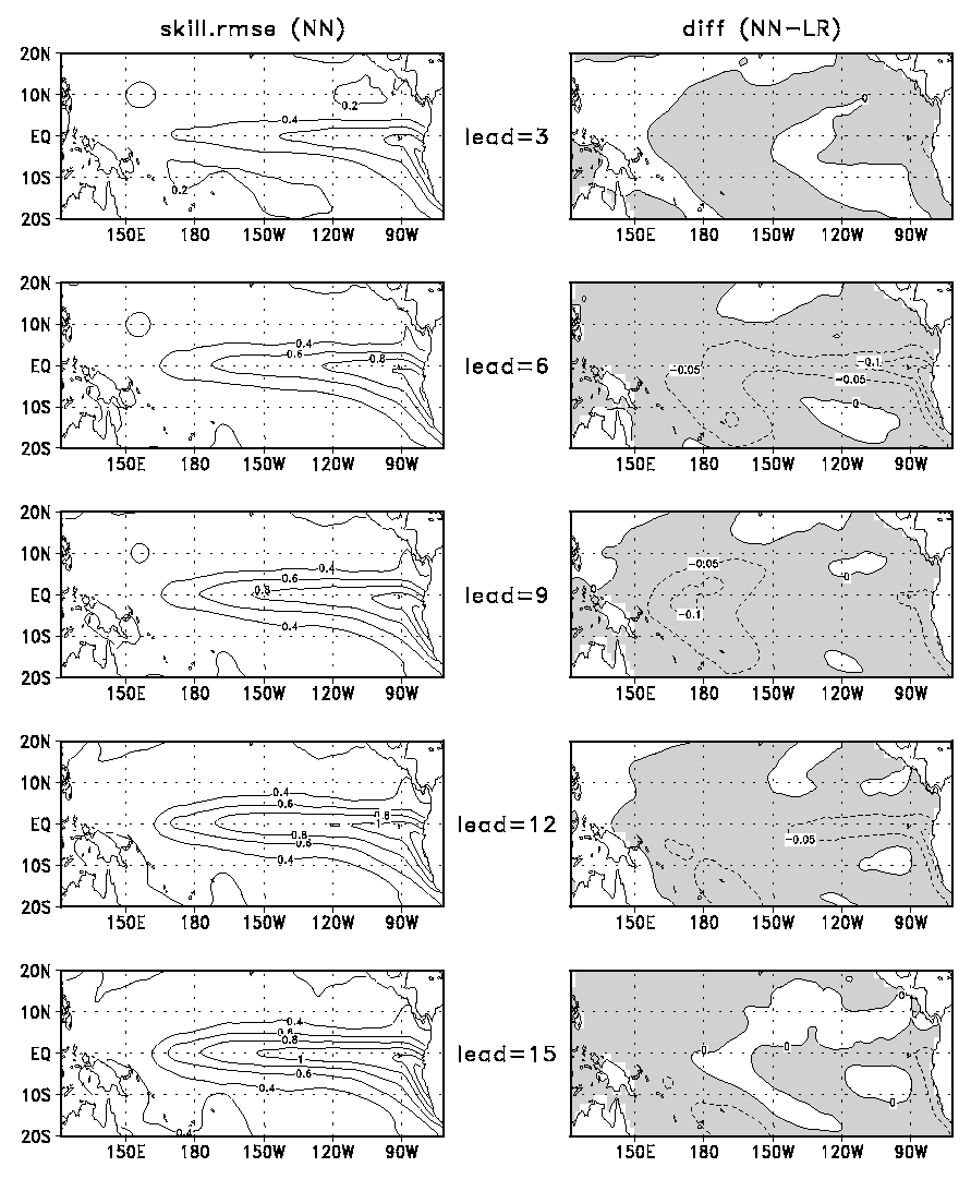
Fig. 3 shows the RMSE (left column) of the NN model at 3-15 month forecast lead times. The difference of the RMSE between the NN model and the linear regression (LR) model (NN minus LR) is shown in the right column. Areas with negative value (NN better than LR) are shaded.
References
Behringer, D. W., M. Ji, and A. Leetmaa, 1998: An Improved coupled model for ENSO prediction and implications for ocean initialization. Part I: The ocean data assimilation system. Mon. Wea. Rev., 126, 1013-1021.
Kalnay, E., et al., 1996: The NCEP/NCAR 40 year reanalysis project. Bull. Amer. Meteo. Soc., 77, 437-471.
Smith, T.M., and R.W. Reynolds, 2004: Improved Extended Reconstruction of SST [1854-1997]. Journal of Climate, 17, 2466-2477.
Tang, B., W.W. Hsieh, A.H. Monahan and F.T. Tangang, 2000. Skill comparisons between neural networks and canonical correlation analysis in predicting the equatorial Pacific sea surface temperatures. J.Climate, 13: 287-293.